Author's Note: This 9th PSpice Tutorial was contributed by Mr. Aminul Siddiqui, an
excellent graduate teaching assistant and student. All I have done to this tutorial is to adapt it
from its original document format to HTML so that it would have a similar look and feel to the other
tutorials. Great job and thanks, Aminul.
William E. Dillon, Ph.D., P.E. June 24, 2006
During a design many parameters are varied to optimize the performance. It can become extremely tedious moving along the response curves to find the exact settling time, power or voltage that optimizes the circuit. A parametric sweep of the parameter "cloud" over the range of values using defined steps can generate the data for the performance analysis, and thus make it simpler to recognize the particular value of the devices that produces optimum response.
One of the most interesting aspects of circuit analysis is the study of Parametric Sweep analysis of Passive Devices using PSpice. It helps to study the DC circuit analysis, Transient analysis, Steady-state AC, and Frequency response with a varying passive device (mostly resistors, capacitors, and inductors) value. To perform these analyses we introduce another group of "dot" commands. It is recommended that you get familiar with tutorials concerning DC and AC analysis, Transient and Frequency response.
The .STEP statement performs a parametric sweep to be performed on a specified variable. This variable can be, for example, a resistance, capacitance, inductor, temperature, etc. If, for example, we wanted to look at how a resistance affected a DC output voltage, we could run the circuit, change the value of resistance, and run the circuit again. This would be repeated over and over. Or we could place the .STEP statement in the PSpice input file, and PSpice would do it automatically for us.
*[Type] <sweep variable name> <model
parameter> <start > <end > <increment>
.STEP RES
RMOD(R) 1,
5,
2
In the statement above, RES is the sweep variable name (a model type), RMOD is the model name, and R is the parameter within the model to step (i.e. the line value). To step the value of the resistor, the line value of the resistor is multiplied by the R parameter value to achieve the final resistance value, that is:
Final resistor value = Line resistor value * R
Therefore, if you set the line value of the resistor to 1 ohm, the final value is 1*R. Thus by stepping R from 1 to 5 ohms will then step the resistor value from 1*1 ohms to 1*5ohms. An added benefit is that you could display all of the results simultaneously in a plot or as a text output.
TYPE: is optional; LIN (linear increments), DEC (increment points per decade), OCT (increment points per octave), STEP defaults to LIN if no sweep type is defined.
The following is a review of useful "DOT" commands discussed in earlier tutorials.
The .MODEL statement defines a set of device parameters for a specific device, which can be referenced in the circuit.
* <model name>
<model variable [model parameters (line value)]>
.MODEL RMOD RES(R=1)
In the statement above, a model type and a model name followed by a model parameter name in parenthesis. The parameter in the model is set to the sweep value.
The .TRAN statement causes a transient analysis to be performed on the circuit. The transient analysis calculates the circuit's behavior over time, always starting at TIME = 0s and finishing at a time specified by the user.
* < print step value > < final time > < print delay> <Max step>
.TRAN 500us 100ms 0s 500us UIC
In the statement above < print step value > is the time interval used for printing or plotting the results of the transient analysis to a specified output file. < final time value > is the ending value of the time interval. Note that the transient analysis always starts off at 0s and ends at the time specified by the final time value. <print delay> is the print delay time this specified value is the no-print value and the results from this value are not plotted, printed, or given to probe. <max step> is the maximum time step size PSpice is allowed to take during the simulation. Since PSpice automatically adjusts its time step size during the simulation, it may increase the step size to a value greater than desirable for displaying the data. When the variables are changing rapidly, PSpice shortens the step size, and when the variables change more slowly, it increases the step size. The last parameter in our list is "UIC." is an acronym for " UseInitialConditions."
The .PROBE statement writes the results from DC, AC, and transient analysis to a data file named PROBE.DAT. It saves information for all voltages and currents. This file can then be called up by the Probe waveform analyzer for graphic display of the results. If we create a circuit listing named "CIRCUIT1.CIR" containing a ".TRAN" statement and a ".PROBE" statement, PSpice will create a file named "CIRCUIT1.DAT" holding the data as well as the usual "CIRCUIT1.OUT" file with basic information about the circuit. By default, the data file created by PSpice is a binary data file; i.e., you can't read it with a text editor.
The .DC command causes the DC sweep analysis to be performed on the circuit. One or more sweep variables are varied over a specific range for specific points. At each point, the DC operating point (all of the DC voltages and currents in the circuit) are calculated.
* < Sweep Variable > <Starting Value > < Stopping Value> <increment>
.DC Vs 20.0 20.0 1.0
For our example problem, we choose the voltage source and set the sweep variable range so that it cannot run more than one value. Since the starting value equals the stopping value, the analysis will only run for one case, i.e., for Vs at 20 volts. Remember that the only reason we are running the DC sweep statement is to enable the .PRINT command.
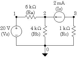
RES_Dc_Analysis
Vs 1 0 DC 20.0V
Ra 1 2 RMOD 1
.MODEL RMOD RES(R=1)
.STEP RES RMOD(R) 1k, 5k, 2k
Rb 2 0 4.0k
Rc 3 0 1.0k
Is 3 2 DC 2.0mA
.DC Vs 20 20 1
.PRINT DC V(1,2) I(Ra)
.END
In the example above, we have three resistors; we can determine the DC analysis (i.e. voltage and current characteristic on each of the node or devices). Here we can step the value of a Resistor (Ra) between 1K to 5K and study the corresponding voltage and current response with the help of the .PRINT command. You may choose to sweep the value of the resistor Rb or Rc in the same manner. The output file "CIRCUIT1.OUT" is shown below, showing the voltage across the node 1 and 2, and the current for the specified values of the Resistor in the .STEP statement.
The output file has been edited to remove the extra lines to obtain the necessary information only. In practice you will find other information pertaining to the analysis.
RMOD R 1
**** 08/09/04 11:34:49 *********** Evaluation PSpice (Nov 1999) **************
RES_Dc_Analysis
**** DC TRANSFER CURVES TEMPERATURE = 27.000 DEG C
**** CURRENT STEP RMOD R = 1.0000E+03 ;(1st sweep value)
Vs V(1,2) I(Ra)
2.000E+01 2.400E+00 2.400E-03
**** 08/09/04 11:34:49 *********** Evaluation PSpice (Nov 1999) **************
RES_Dc_Analysis
**** DC TRANSFER CURVES TEMPERATURE = 27.000 DEG C
**** CURRENT STEP RMOD R = 3.0000E+03 ;(2nd sweep value)
Vs V(1,2) I(Ra)
2.000E+01 5.143E+00 1.714E-03
**** 08/09/04 11:34:49 *********** Evaluation PSpice (Nov 1999) **************
RES_Dc_Analysis
**** DC TRANSFER CURVES TEMPERATURE = 27.000 DEG C
**** CURRENT STEP RMOD R = 5.0000E+03 ;(3rd sweep value)
Vs V(1,2) I(Ra)
2.000E+01 6.667E+00 1.333E-03
JOB CONCLUDED
TOTAL JOB TIME .02
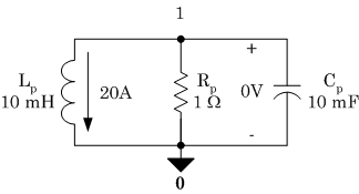
RES_TRANSIENT
R 0 1 RMOD 1
.MODEL RMOD RES(R=1)
.STEP RES RMOD(R) 1, 5, 2
Rp 1 0 Rmod 1
Lp 1 0 8mH IC=20A
Cp 1 0 10mF IC=0V
.TRAN 500US 100MS 0S 500US UIC
.PROBE
.END
In the above example, the Resistor value is swept between 1ohm and 5ohms with an increment of 2. The eight millihenry inductor, Lp, has an initial current of 20 amps flowing from node 1 through the inductor to node 0. The 10 millifarad capacitor, Cp, has an initial voltage of 0 volts. Both the print step size and the maximum step size are set to 500?s and the final time is 100ms. There is no print delay, and PSpice is instructed to use the initial conditions provided.
The output file ""RES_CIR.OUT" is shown below.
**** 08/07/04 14:23:36 *********** Evaluation PSpice (Nov 1999) **************
RES_TRAN
Rp 0 1 RMOD 1
.MODEL RMOD RES(R=1)
.STEP RES RMOD(R) 1,5,2
Lp 1 0 8mH IC=20A
Cp 1 0 10mF IC=0V
.TRAN 500US 100MS 0S 500US UIC
.PROBE
.END
**** Resistor MODEL PARAMETERS
RMOD
R 1
JOB CONCLUDED
TOTAL JOB TIME .13
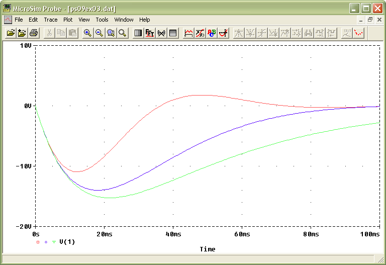
For meaningful information about the transient response we need to use another program that is bundled with PSpice. This program is named PROBE. You can launch Probe from the Start menu of Windows, but you will then need to go to Probe's File menu and open the DAT file you want to see. After you have Probe running with the proper DAT file open, choose "Add" in the Probe Trace menu. You will see a list of circuit variables that can be displayed. Choose V2(R), the voltage at node 1, and then click "OK." You should see the following trace in Probe.
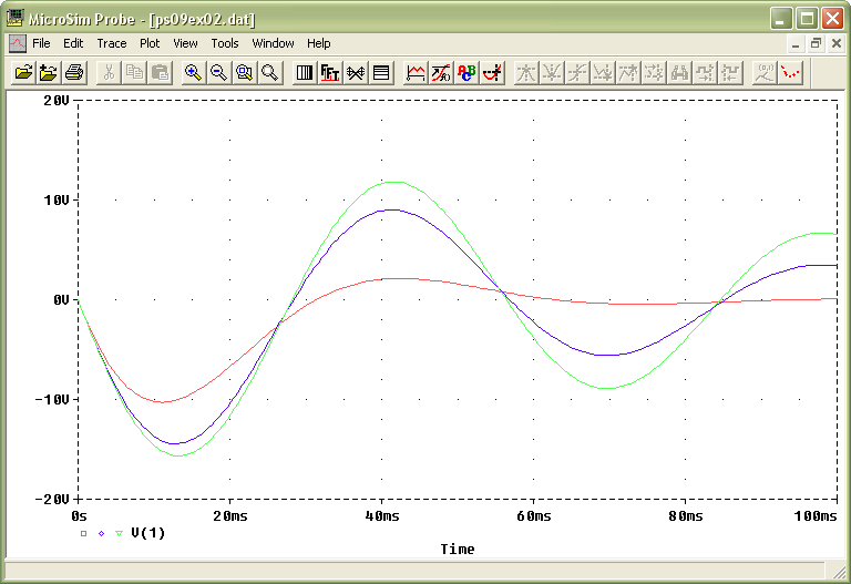
Each of the curves above represents the three Resistor values specified in the .STEP statement. (Right click on a curve, click on information to see the corresponding value of the Resistor). In Probe, click on the V2(R) at the lower left corner and then hit the "Delete" key. Then go to Trace menu in the Probe and choose "Add" again. This time choose I2(R) and click "OK". You should be able to see the transient current response for the three different Resistors sweep values.
Similarly, in another example you can decide to sweep the Capacitor and Inductor values using the .STEP statement to study the transient analysis of the RLC circuit. The second example shows the sweep of the Inductor values of our RLC circuit. The parameter of the .STEP command stays the same, only the .MODEL statement has changed to an Inductor.
IND_TRANSIENT
Rp 0 1 1
Lp 1 0 LMOD 1 IC=20A
.MODEL LMOD IND (L=10mH)
.STEP IND LMOD(L) 10mH, 50mH, 20mH
Cp 1 0 10mF IC=0V
.TRAN 500US 100MS 0S 500US UIC
.PROBE
.END
In the above example, the value of the Resistor and Capacitor is kept constant, while sweeping the Inductor value between 10mH and 50mH with a step size of 20mH. You should see the following transient analysis of the voltage across the inductor using the trace in Probe.
In Probe, click on the V1 at the lower left corner and then hit the "Delete" key. Then go to Trace menu in the Probe and choose "Add" again. This time choose I(L) and click "OK". You should be able to see the transient current response for the three different Inductor sweep values.
We have learned about the Steady-State AC analysis in PSpice from tutorial no 5. This section is a continuation of the example with an added feature of the device sweep. To see the results of this analysis in the .OUT file, we will want to use a new form of the .PRINT command. The .PRINT statement allows results from DC, AC, noise, and transient analysis to be output in the form of tables, referred to as print tables. In the first tutorial, we learned that the .PRINT DC command would not work unless we enabled it with the .DC command. In this case we will use the .AC command to enable the .PRINT AC command to print our phasor voltages and currents in the output file.
Here is an example of circuit operating at 60Hz, with three passive devices. The idea is to sweep the devices using the .STEP command, and study the AC response.
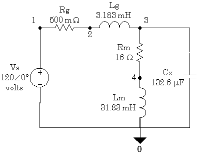
RES_AC_ANALYSIS 60Hz
Vs 1 0 AC 120V 0
Rg 1 2 RMOD 1
.MODEL RMOD RES(R=1)
.STEP RES RMOD(R) 0.5, 5, 2
Lg 2 3 3.183mH
Rm 3 4 16.0
Lm 4 0 31.83mH
Cx 2 0 132.6uF
.AC LIN 1 60 60
.PRINT AC VM(Rg) VP(Rg) IM(Rg) IP(Rg)
.END
The output file of the simulation is shown below. Only the relevant steady-state analysis information due to the Resistor sweep between the values of 0.5ohms to 4.5ohms is shown. In practice the "RLCNA.OUT" will carry addition information of the simulation. It has been edited to remove extra lines. Note that the output file shows the voltage and current magnitude for the three Resistor sweep values.
************************************************************************
RMOD R 1
**** 08/08/04 12:27:16 *********** Evaluation PSpice (Nov 1999) **************
RES_ACANALYSIS 60Hz
**** AC ANALYSIS TEMPERATURE = 27.000 DEG C
**** CURRENT STEP RMOD R = .5 ;(1st sweep value)
************************************************************************
FREQ VM(Rg) VP(Rg) IM(Rg) IP(Rg)
6.000E+01 1.234E+00 2.690E+01 2.468E+00 2.690E+01
**** 08/08/04 12:27:16 *********** Evaluation PSpice (Nov 1999) **************
RES_ACANALYSIS 60Hz
**** AC ANALYSIS TEMPERATURE = 27.000 DEG C
**** CURRENT STEP RMOD R = 2.5 ;(2nd sweep value)
************************************************************************
FREQ VM(Rg) VP(Rg) IM(Rg) IP(Rg)
6.000E+01 5.745E+01 2.491E+01 2.298E+00 2.491E+01
**** 08/08/04 12:27:16 *********** Evaluation PSpice (Nov 1999) **************
RES_ACANALYSIS 60Hz
**** AC ANALYSIS TEMPERATURE = 27.000 DEG C
**** CURRENT STEP RMOD R = 4.5 ;(3rd sweep value)
************************************************************************
FREQ VM(Rg) VP(Rg) IM(Rg) IP(Rg)
6.000E+01 9.665E+01 2.318E+01 2.148E+00 2.318E+01
JOB CONCLUDED
TOTAL JOB TIME .02
In a similar example you can decide to sweep the Capacitor and Inductor values using the .STEP statement to study the Steady-state AC analysis of the RLC circuit. The second example shows the sweep of the Inductor value of the RLC circuit. The parameter of the .STEP command stays the same, only the .MODEL statement has changed to an Inductor.
IND_AC_ANALYSIS 60Hz
Vs 1 0 AC 120V 0
Rg 1 2 0.5
Lg 2 3 LMOD 1
.MODEL LMOD IND(L=1mH)
.STEP IND LMOD(L) 1mH, 5mH, 2mH
Rm 3 4 16.0
Lm 4 0 31.183mH
Cx 2 0 1uF
.AC LIN 1 60 60
.PRINT AC VM(Lg) VP(Lg) IM(Lg) IP(Lg)
.END
The output file of the simulation is shown below. Only the relevant steady-state analysis information due to the Inductor sweep between the values of 1mH to 5mH for the steady-state analysis is shown. In practice the "RLCNA.OUT" will carry addition information of the simulation. Note that the output file shows the voltage and current magnitude for the three Inductor sweep values.
LMOD
L 1.000000E-03
**** 08/08/04 13:11:18 *********** Evaluation PSpice (Nov 1999) **************
IND_ACANALYSIS 60Hz
**** AC ANALYSIS TEMPERATURE = 27.000 DEG C
**** CURRENT STEP LMOD L = 1.0000E-03 ;(1st sweep value)
************************************************************************
FREQ VM(Lg) VP(Lg) IM(Lg) IP(Lg)
6.000E+01 2.209E+00 5.366E+01 5.859E+00 -3.634E+01
**** 08/08/04 13:11:18 *********** Evaluation PSpice (Nov 1999) **************
IND_ACANALYSIS 60Hz
**** AC ANALYSIS TEMPERATURE = 27.000 DEG C
**** CURRENT STEP LMOD L = 3.0000E-03 ;(2nd sweep value)
FREQ VM(Lg) VP(Lg) IM(Lg) IP(Lg)
6.000E+01 6.482E+00 5.200E+01 5.732E+00 -3.800E+01
**** 08/08/04 13:11:18 *********** Evaluation PSpice (Nov 1999) **************
IND_ACANALYSIS 60Hz
**** AC ANALYSIS TEMPERATURE = 27.000 DEG C
**** CURRENT STEP LMOD L = 5.0000E-03 ;(3rd sweep value)
************************************************************************
FREQ VM(Lg) VP(Lg) IM(Lg) IP(Lg)
6.000E+01 1.057E+01 5.041E+01 5.605E+00 -3.959E+01
JOB CONCLUDED
TOTAL JOB TIME .01
The purpose of this type of analysis is to study the frequency response of different kinds of circuits. Since frequency sweeps produce a lot of data that needs to be graphed to be clearly understood, we will reintroduce Probe, the graphing program that is bundled with PSpice. In order to sweep the frequency we need to use the .AC command. The .AC statement is used to calculate the frequency response of a circuit over a range of frequencies. In addition to the frequency sweep, we will sweep the passive devices in the circuit, to simply recognize the particular value of the devices that produces optimum response.
As in tutorial no 7, we will use a second-order high pass filter to sweep the value of the Resistor over a range of frequency to study its response.
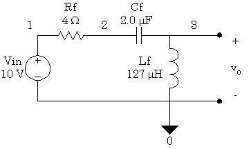
RES_FREQUENCY RESP. SECOND ORDER HIGH PASS FILTER
Vs 1 0 AC 10V 0
Rf 1 2 RMOD 1
.MODEL RMOD RES(R=4)
.STEP RES RMOD(R) 4, 8, 2
Cf 2 3 2uF
Lf 3 0 127uH
.AC DEC 20 100Hz 1MEG
.PROBE
.END
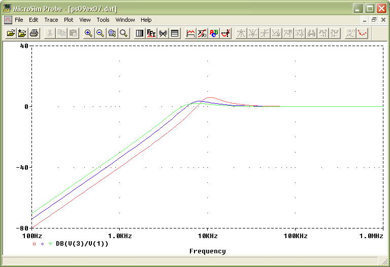
This time also we did not use 1V for the input voltage. Therefore, we will need to have PROBE actually divide the input into the output to get the gain. We show this gain in decibels. (To learn about gain plots in decibels please refer back to tutorial no 7)
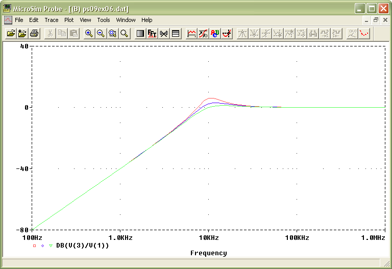
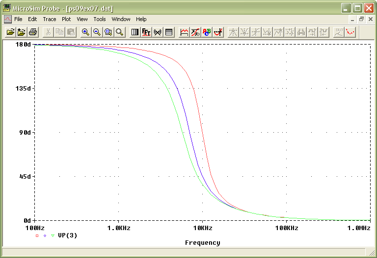
Notice that the gain below the resonant frequency of 10 kHz slopes upward at 40 dB/decade. We show this gain in decibels by dividing the input into the output.
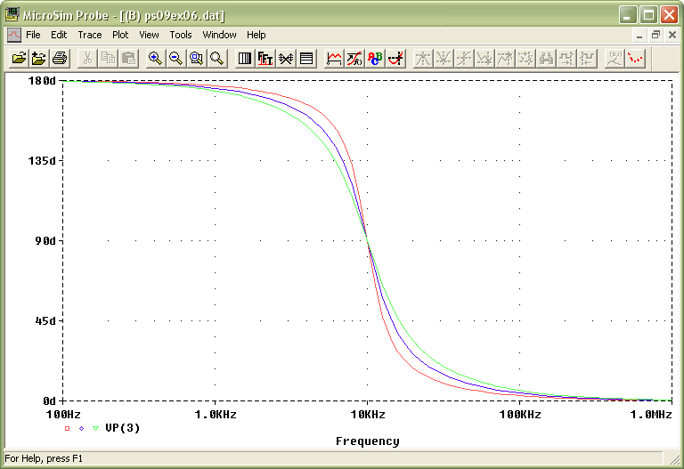
When we plot the phase shift of this filter, we only need to specify the phase angle of the output voltage since the input voltage was specified at 0 degrees.
In a similar example we can decide to sweep the Capacitor and Inductor values using the .STEP statement to study the Steady-state AC analysis of the RLC circuit. The second example shows the sweep of the capacitor value of the second-order high pass filter circuit. The parameter of the .STEP command is the same, only the .MODEL statement has changed to a Capacitor.
CAP_FREQUENCY RESP. SECOND ORDER HIGH PASS FILTER
Vs 1 0 AC 10V 0
R 1 2 4
C 2 3 CMOD 1
.MODEL CMOD CAP(C=2uF)
.STEP CAP CMOD(C) 2uF, 6uF, 2uF
L 3 0 127uH
.AC DEC 20 100Hz 1MEG
.PROBE
.END
We only need to specify the phase angle of the output voltage since the input voltage was specified at 0 degrees.