Up to now, these tutorials have discussed only the most basic types of sources. These include the independent DC and AC voltage and current sources, and the simple voltage or current controlled dependent voltage and current sources. At this time, we will introduce three new independent source types and two new dependent source types. This by no means completes the list of possible sources in PSpice, but these new sources will add a great deal of capability to our circuit modeling efforts.
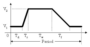
This type of source can be either a voltage or a current source. We often use it as a stimulus for transient response simulation of a circuit. It should never be used in a frequency response study because the model assumes it is in the time domain. The designation of the pulse source starts as any other independent source; i.e., the part name must begin with the letter V (for voltage) or I (for current). This is followed by the node names. Then, instead of "DC" or "AC," we use the keyword "PULSE" followed by the necessary parameter list. Items in the parameter list may be separated by spaces or commas. An example of a pulse type of voltage source follows:
The parameters for the pulse (to be entered in the order given) are:
A case study now follows for a simple circuit with a pulsed source:
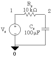
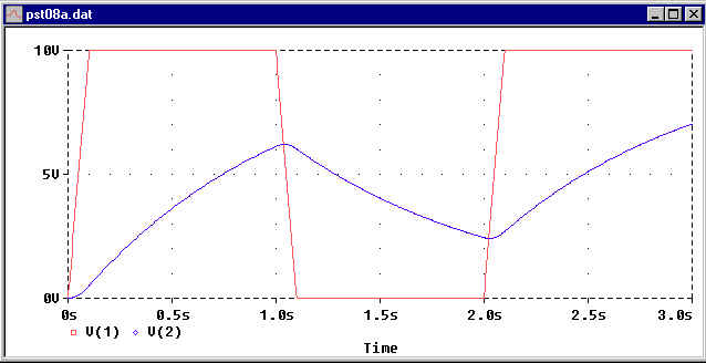
Transient response of a low-pass filter
* V1 V2 Td
Tr Tf Tw Per.
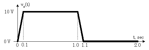
Vs 1 0 PULSE(0V 10V 0s 100ms 100ms 900ms 2s)
Rs 1 2 10k
Cs 2 0 100uF IC=0V
.TRAN 5ms 3s 0s 5ms UIC
.PROBE
.END
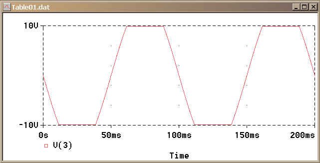
Discussion: V1 is set to zero for this case and the pulse is at the 10-volt level (V2) for Tw = 900 ms. Note that the simulation time (3s) is greater than the period (2s). The red trace shown below represents the pulse from the voltage source while the blue trace represents the response voltage across the capacitor.
The SIN type of source is actually a damped sine with time delay, phase shift and a DC offset. Usually, we only want a simple sine wave to model an AC power source in a transient analysis simulation. For the record, here is the whole definition with all six parameters explained. The following represents a voltage source, but the first two parameters could readily be changed to currents in amps to make this a current source. N. B.: Do not use this type of source for a phasor or frequency sweep analysis.
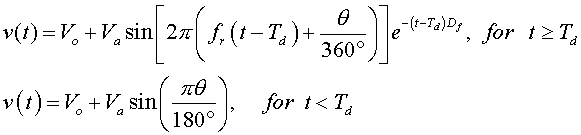
Below is a sample waveform where: Vo = 2V, Va = 5V, Fr = 2Hz, Td = 200ms, Df = 2s-1 and θ = 30°.
Here is the circuit listing that produced the above waveform:
Example of a SIN source
* Vo Va Fr Td Df θ
Vs 1 0 SIN(2V 5V 2Hz 200ms 2Hz 30d)
RS 1 0 1MEG
.TRAN 1ms 2s 0s 1ms UIC
.PROBE
.END
The way PSpice uses the parameters is:
Now that we got that out of the way, let's see an example of a plain sinusoid as it may be used in a power system transient response simulation.
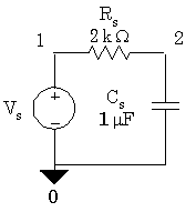
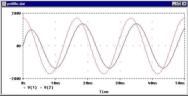
Let the above circuit commence with a cosine waveform starting at t = 0. There is no stored energy in the capacitor. The input data for this circuit would be:
Transient Response of a Sinusoid
* Vo Va Fr Td Df θ
Vs 1 0 SIN(0V 170V 60Hz 0s 0Hz 90d)
RS 1 2 2k
Cs 2 0 1uF IC=0V
.TRAN 100us 50ms 0s 100us UIC
.PROBE
.END
Note that the normal usage of this source type is to set Vo, Td and Df to zero. Since a cosine was required here, we set the phase advance to 90 degrees. If we were willing to use a sine instead of a cosine, the last three parameters would have been equal to zero and could have been omitted. The Probe output for this case is shown below. The red waveform is the cosine source voltage and the blue waveform is the capacitor response voltage.
The PWL source is a PieceWise Linear function that you can use to create a waveform consisting of straight line segments drawn by linear interpolation between points that you define. Since you can use as many points as you want, you can create a very complex waveform. This source type can be a voltage source or a current source. Like all the other independent sources, the part name must start with the letter "V" for a voltage source and the letter "I" for a current source. The syntax for this source type is flexible and has several optional parameters. The required parameters are two-dimensional points consisting of a time value and a voltage (or current) value. There can be many of these data pairs, but the time values must be in ascending order, and the intervals between time values need not be regular. The two optional parameters are "DC" and "AC." The use of an AC parameter with this source is very dubious since it is intended for use with transient analyses, and any AC value would be ignored. However, if you want to change the analysis type and use an AC source the AC parameter would be the only thing used.
Let's examine a few examples of this source type:
* +n -n dc=10 ac=1
point 2 point 3 point 4
Vx 12 24 DC 10V AC 1V PWL(1ms 12V 3ms 15V 8ms 4V)
In the above example, the AC parameter will be ignored in a transient analysis. The DC parameter will be paired with time = 0s to create the first data point. If, for some peculiar reason, you run an AC sweep with this source, it would be a simple 1V AC source at the frequencies designated. An equivalent usage of this source that is more clear will now be presented.
* +n -n point 1 point 2 point 3 point 4
Vx 12 24 PWL(0ms 10V 1ms 12V 3ms 15V 8ms 4V)
Note that we have discarded the unneeded AC parameter and obviated the need for the DC parameter by entering the starting point in the PWL list. Additional flexibility exists in the various ways PSpice will accept parameter lists. We can use commas, spaces or tabs as we wish; and the parentheses enclosing the parameter lists are not required. Here are a few examples that are equivalent to the first two.
Vx 12 24 PWL 0ms,10V 1ms,12V 3ms,15V 8ms,4V; <== no ()
Vx 12 24 PWL(0ms,10V,1ms,12V,3ms,15V,8ms,4V)
Vx 12 24 PWL(0ms,10V 1ms,12V 3ms,15V 8ms,4V)
If the time span of the transient analysis exceeds the time value of the last point, the source behaves as a DC source set at the voltage (or current) value of the last point for the rest of the simulation. It does not repeat its cycle as does the Pulse source.
Finally, we will create an example using a simple PWL source:
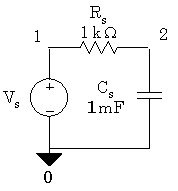
PWL Example
Vs 1 0 PWL(0s,5V 1s,8V 2s,10V 3s,2v)
RS 1 2 1.0k
Cs 2 0 1mF IC=0V
.TRAN 1ms 5s 0s 1ms UIC
.PROBE
.END
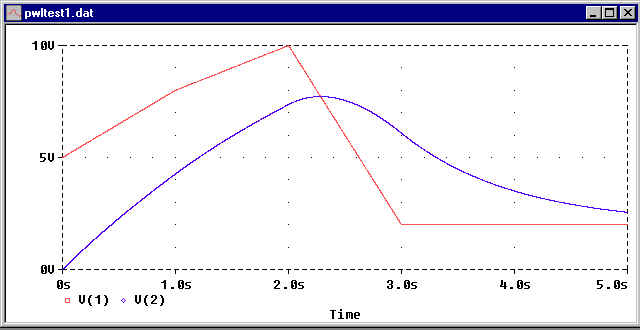
In the above figure, the red trace is the source waveform we created and the blue waveform is the response voltage across the capacitor.
Although there are several more independent source types, the exponential and SFFM sources to mention a couple, we will postpone their explanation until a future tutorial. At this point, we will benefit more from the understanding of two new dependent source types: the Laplace dependent source and the Table dependent source.
The Laplace source is a transfer function actuator. It takes a mathematical expression of circuit voltages or currents as its input and produces its output on the basis of the transfer function defined in the Laplace domain. This can replace the detailed modeling of the circuit which accomplishes the same thing. This source is usually used for frequency response filter modeling, but also works in the time domain. A Laplace source can be an expression-controlled voltage source or an expression-controlled current source. The expression can be a function of the voltage between a pair of nodes or the current flowing through a voltage source. Usually, we just use a node voltage as the input expression.
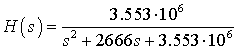
Suppose we have a transfer function, H(s), defined in the Laplace domain as:
![]()
This could represent a low-pass filter with a cutoff frequency of 1000 radians/sec (or 159 Hz). The elements used to model this in a circuit application could appear as follows:
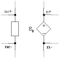
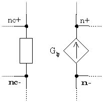
In the above circuit fragment, the input is the voltage drop from node nc+ to nc- and the output appears as the dependent source voltage at element Elp. The input code that will reside in the circuit file would be:
* input transfer
function
Elp n+ n- LAPLACE {V(NC+,NC)}={1000/(s+1000)}
An interesting quirk of this source is that there must be a space immediately to the right of the keyword "LAPLACE" and before the left curly brace that starts the input expression. Another quirk is that the transfer function enclosed in curly braces must reside on one line. Also notice how the transfer function is encoded.
The current source version of this source could be:
The circuit file data for the above fragment would be:
* input transfer
function
Glp n- n+ LAPLACE {V(NC+,NC)}={1000/(s+1000)}
Now, we will construct an actual example of the Laplace source used as a filter tester. The transfer function is for a two-pole low-pass Butterworth filter with a corner frequency of 300 Hz.
A minimal circuit to test this filter is shown below.
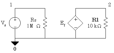
The circuit file code to model the above circuit is shown below. We will let the frequency sweep span three decades. Note the method for encoding the transfer function as an inline statement. This is not unlike a line of programming code.
Laplace Example
Vs 1 0 AC 1V
RS 1 0 1MEG
Ef 2 0 Laplace {V(1)}={3.553E6/(s^2+2666*s+3.553E6)}
Rl 2 0 10k
.AC DEC 20 10Hz 10kHz
.PROBE
.END
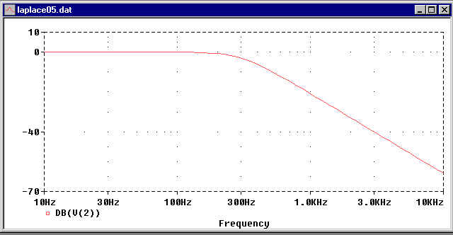
Now, we will examine the Bode plot for this filter as produced by PROBE.
To demonstrate that the Laplace source can work well in the time domain, we excite the same filter with a pulse instead of a frequency sweep. The circuit file code for this is:
Laplace Transient Example
Vs 1 0 PULSE(0V 10V 0s 10us 10us 4.99ms 10ms)
RS 1 0 1MEG
Ef 2 0 Laplace {V(1,0)}={3.556E6/(s^2+2666*s+3.553E6)}
Rl 2 0 10k
.TRAN 1us 10ms 0s 1us
.PROBE
.END
And the results from PROBE are:
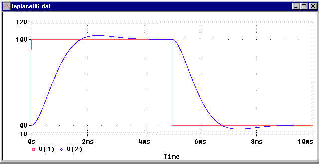
where the red trace is the input pulse and the blue trace is the filter output response.
The Laplace source allows us to model complex electromechanical systems or control systems in terms of the block diagrams where the transfer functions are known. There is no need to define the complex circuitry within the block. However, it should be noted that the Laplace source makes heavy use of resources. There is a price for the convenience.
This source type is one of the most flexible and powerful modeling methods offered by PSpice. It is a dependent source because its output is dependent on the voltages or currents used in the input expression. Instead of a mathematical function, a lookup from a table of points is executed from the input expression. Linear interpolation is used whenever the input expression's value lies between two table values. Consider the following graph:
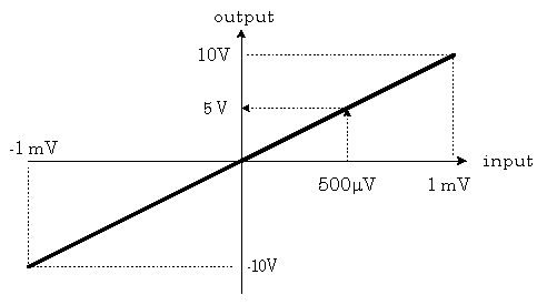
Only two points are needed to specify this graph: (-1mV, -10V) and (1mv, 10V). Any input value between -1mV and +1mV has a corresponding value from the graph. For example, an input value of 500mV would produce an output voltage of 5V. The way PSpice interprets the table data, an input value outside the defined range will simply return the closest output value; i.e., an input value of 2mV would still return 10V for the output. If we examine this graph in its linear region, we find a ratio of 104 between output and input. Thus our graph describes a gain of 104 between the range of -1mV to +1mV of input. We could use this to define an op-amp with an open loop gain of 104 that saturates at 10 volts. Here is how we could encode this Table type voltage source in a PSpice circuit file:
* n+ n- input
in out in out
Etab 2 0 TABLE {V(1)}=(-1mV,-10V) (1mv,10V)
where the voltage at node 1 is the input. Note that the table data pairs require an input value, then an output value. Grouping the data pairs with parentheses and commas as shown above is strictly for human convenience. PSpice allows a great deal of stylistic freedom in accepting tabular data. One quirk you must remember, however, is that a space is required between the keyword "TABLE" and the left curly brace that starts the input expression. This is similar to the Laplace source syntax requirements. You may use continuation lines for the input/output data pairs. Since linear interpolation is used between data pairs, these data pairs must be ordered so that the input values are in ascending order.
Now, we will define an opamp subcircuit using this source with a 500 kΩ input resistance and a 50 Ω output resistance:
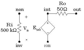
.SUBCKT OpAmpSat non inv out com
Ri non inv 500k
Ro int out 50.0
Et int com TABLE {V(non,inv)}=(-1mV,-10V) (1mV,10V)
.ENDS
Due to the saturation effects enabled by the TABLE paradigm, this subcircuit will behave as an opamp whose +Vcc and -Vcc values are +10V and -10V respectively. Let's try it out in an inverting amplifier circuit. We will overdrive the input with a SIN source to see the saturation effects.
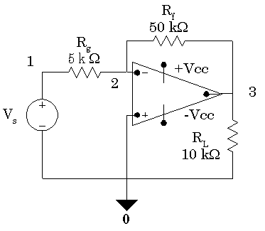
Saturated Opamp Example
Vs 1 0 SIN(0V 1.5V 10Hz); last 3 params = 0
Rg 1 2 5k
Rf 2 3 50k
RL 3 0 10k
Xp 0 2 3 0 OpAmpSat; must include above subckt def.
.TRAN 100us 200ms 0s 100us
.PROBE
.END
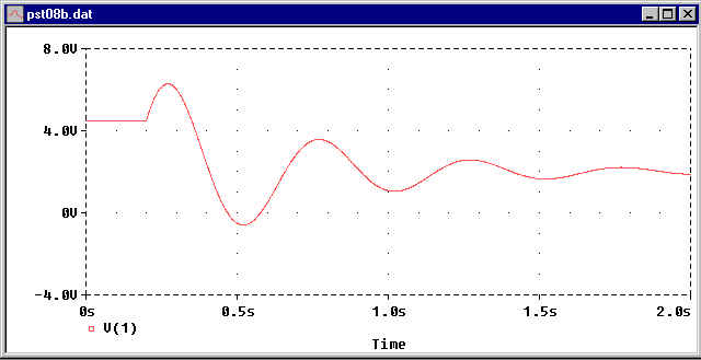
The output voltage from PROBE is shown below:
The closed loop gain of this inverting amplifier circuit is -10. Since the peak input voltage is 1.5V, the output peaks would be 15V were it not for the saturation effect. This opamp circuit uses far less resources than the somewhat more accurate library models included with PSpice.
A more sophisticated example of an input/output table follows:
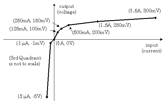
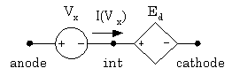
The above graph is an approximate representation of the v-i characteristic of a diode. We can create a diode model from a Table type dependent voltage source whose input is the current through the diode branch. To do this, we will need to resort to the old trick of using a zero-value DC voltage source to measure the current. The elements would be connected as follows:
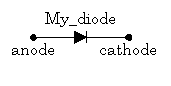
We'll create a subcircuit for our diode model:
.SUBCKT My_diode anode cathode
Vx anode int DC 0V; use this to measure current
Ed int cathode TABLE {I(Vx)}=(-2uA,-5V) (-1uA,-1mV)
+ (0A,0V) (125mA,100mV) (250mA,150mV) (500mA,200mV)
+ (1.5A,250mV) (3.5A,300mV)
.ENDS
Now let's test our diode subcircuit in a simple half-wave rectifier circuit.
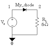
Diode Simulation with Table
Vs 1 0 SIN(0V 6V 10Hz)
Rl 2 0 5.0
Xd 1 2 My_diode; must include above SUBCKT
.TRAN 100us 200ms 0s 100us
.PROBE
.END
The PROBE plot for this simulation follows.
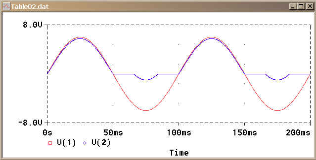
The red trace represents the 6-volt peak-value sine wave and the blue trace represents the voltage across the load resistor. The voltage difference between the two traces during the positive half-cycles is the forward voltage drop across the diode. Since the largest negative voltage given in the table was only 5 volts, there is a Zener breakdown when the diode's reverse voltage exceeds 5 V. If you do not wish to model the Zener diode breakdown effect, simply set the output value of the first data pair in the table to a large enough negative value. Bear in mind, that the diode models included in the PSpice library are more sophisticated than this, but they require more resources.
Although these two TABLE source examples did not utilize the current source capability, you can easily create Table-type current sources by replacing "E" by "G" in the part name and remembering that the output values in the data pairs have become currents.
There are almost limitless possibilities for modeling electronic parts with these sources.