In addition to DC circuit analysis and transient analysis, PSpice can be used to work steady-state phasor problems. To see the results of this analysis in the .OUT file, we will want to use a new form of the .PRINT command. In the first tutorial, we learned that the .PRINT DC command would not work unless we enabled it with the .DC command. This was the DC sweep command although we only allowed it to sweep a single value of voltage. We have a somewhat similar situation when we need to print AC values; i.e., we will use the .AC command to enable the .PRINT AC command to print our phasor voltages and currents.
Up to now, all our voltage and current sources were DC. We learned the syntax of the DC source in the first tutorial. The syntax for an AC source is very similar. The AC source is assumed to be a cosine waveform at a specified phase angle. Its frequency must be defined in a separate ".AC" command that defines the frequency for all the sources in the circuit. The unique information for the individual source is: the name, which must start with "V" or "I," the node numbers, the magnitude of the source, and its phase angle. Some examples follow.
*name nodelist type value phase(deg)
Vac 4 1 AC 120V
30
Vba 2 5 AC 240
; phase angle 0 degrees
Ix 3 6 AC 10.0A
-45 ; phase angle -45 degrees
Isv 12 9 AC 25mA
; 25 milliamps @ 0 degrees
Notice that the type, AC, must be specified, because the default is DC. If the phase angle is not specified it will be assumed as zero degrees. The units of the phase angle will be in degrees. As before, the "V" after the voltage value is optional, as is the "A" after the current value in a current source. The polarity of the AC voltage source is determined as if the voltage were a cosine function of ωt at t = 0. Then the node on the left is the positive node and the node on the right is the negative node. Similarly, the polarity of the AC current source is determined as if the current were a cosine function of ωt at t = 0. Then positive current flows into the source from the node on the left, passes through the source, and leaves the source from the node on the right.
A note of caution is needed here. By now, some of you may have discovered the "SIN" type of source by reading some of the supplementary material. The SIN is one of several useful source types (also EXP, PULSE, PWL & SFFM to name a few) that are used for transient analysis. Do not attempt to use SIN for steady-state (phasor) AC analysis nor for frequency sweeps. The SIN type is a time-based function for time-based analysis, whereas the AC type is used in frequency-based modeling. Since phasor analysis uses frequency-based models of circuit elements, always use the AC type as described in this tutorial for phasor analysis of circuits.
Before the .PRINT command will work, it must be enabled by the .AC command. The .AC command was designed to make a sweep of many frequencies for a given circuit. This is called a frequency response and will be discussed in a later tutorial. Three types of ranges are possible for the frequency sweep: LIN, DEC and OCT. At this time we only want a single frequency to be used so it does not matter which one we choose. We will pick the LIN (linear) range to designate our single frequency. Some examples of the .AC statement follow.
* type #points start stop
.AC LIN 1 60Hz 60Hz;
<== what we want now.
.AC LIN 11 100 200;
<== a linear range sweep
.AC DEC 20 1Hz 10kHz;
<== a logarithmic range sweep
The first statement above performs a single analysis using the frequency of 60 Hz. Placing the units "Hz" after the value is optional. The second statement would perform a frequency sweep using frequencies of 100Hz, 110Hz, 120Hz, 130Hz, 140Hz, 150Hz, 160Hz, 170Hz, 180Hz, 190Hz and 200Hz. This will not be used here. The third statement performs a logarithmic range sweep using 20 points per decade over a range of four decades. This will be useful later for studying frequency response of circuits.
Finally, we can discuss the actual .PRINT AC command. Printing the components of phasor values (complex numbers) requires some options. There are four expressions needed for this: magnitude, phase (angle), real part, and imaginary part. In addition, we can print voltages or currents. For instance, to print the magnitude of a voltage between nodes 2 and 3, we would specify "VM(2,3)." The phase angle of this same voltage would be "VP(2,3)" and would be printed in degrees. If we need the current magnitude through resistor Rload, we would specify "IM(Rload)." The real part of the voltage on node 7 would be specified "VR(7)" and its imaginary part, "VI(7)." As with the .PRINT DC command, there is no limit on the number of times it can be used in a listing; nor is there a limit on how many print requests can be on a single line. Some complete examples follow:
.PRINT AC VM(30,9) VP(30,9); magnitude & angle of voltage
.PRINT AC IR(Rx) II(Rx); real & imag. parts Rx current
.PRINT AC VM(17) VP(17) VR(17) VI(17); the whole works on node 17
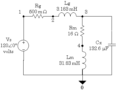
We will analyze the following circuit at a frequency of 60 Hz.
60 Hz AC Circuit
Vs 1 0 AC 120V 0
Rg 1 2 0.5
Lg 2 3 3.183mH
Rm 3 4 16.0
Lm 4 0 31.83mH
Cx 3 0 132.8uF
.AC LIN 1 60 60
.PRINT AC VM(3) VP(3) IM(Rm) IP(Rm) IM(Cx) IP(Cx)
.END
In the above listing, the .AC command sets up the analysis for a single solution at 60 Hz. The .PRINT AC command tells PSpice to report on the voltage magnitude and phase angle at node 3, and the current magnitude and phase angle for the current through resistor Rm and the current magnitude and phase angle through capacitor Cx. The resulting output file (edited to delete clutter) follows:
60 Hz AC Circuit
**** CIRCUIT DESCRIPTION
Vs 1 0 AC 120 0
Rg 1 2 0.5
Lg 2 3 3.183mH
Rm 3 4 16.0
Lm 4 0 31.83mH
Cx 3 0 132.6uF
.AC LIN 1 60 60
.PRINT AC VM(3) VP(3) IM(Rm) IP(Rm) IM(Cx) IP(Cx)
60 Hz AC Circuit
**** SMALL SIGNAL BIAS SOLUTION
TEMPERATURE = 27.000 DEG C
NODE VOLTAGE NODE VOLTAGE NODE VOLTAGE
( 1) 0.0000 ( 2) 0.0000 ( 3) 0.0000
NODE VOLTAGE ( 4) 0.0000
VOLTAGE SOURCE CURRENTS
NAME CURRENT
Vs 0.000E+00
TOTAL POWER DISSIPATION 0.00E+00 WATTS
60 Hz AC Circuit
**** AC ANALYSIS TEMPERATURE = 27.000 DEG C
FREQ VM(3) VP(3)
IM(Rm) IP(Rm)
6.000E+01 1.203E+02 -3.332E+00 6.014E+00 -4.020E+01
FREQ IM(Cx) IP(Cx)
6.000E+01 6.013E+00 8.667E+01
JOB CONCLUDED TOTAL JOB TIME .26
Notice that the small signal bias solution yields zero for the voltages.
This is the DC part of the solution which is zero in this case because there
was no DC excitation. The AC analysis has been printed in blue.
The voltage at node 3 is 120.3 -3.332°
volts and the current through the capacitor is
6.01486.67°
amps. Theory predicts that the current through a capacitor leads
the voltage across the capacitor by 90°, which it does.
-3.332°
volts and the current through the capacitor is
6.01486.67°
amps. Theory predicts that the current through a capacitor leads
the voltage across the capacitor by 90°, which it does.